
A mysterious and longstanding practice of taking the square root of SiLog loss without mention of cause or origin has swept across repositories for monocular depth estimation models, often in conflict with the loss formulations found in the corresponding publications. After careful investigation, the original source and reasoning for this modification remains unknown, so this article seeks to fill in the gap in discussion by exploring theoretical pros and cons for this addition in the context of SiLog loss and monocular depth estimation, and provide experimental support to see how the theory plays out in practice.
In conclusion, the potential advantages of adding this operation do not seem to outweigh the risks of exploding gradients near zero destabilizing weight convergence, and simply increasing the learning rate or loss weight (in the case of multiple losses) is a safer alternative to get more activity from the gradients during training. If you or anyone you know can add more insight to this investigation, please leave a comment!
Background
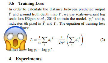
SiLog loss is short for scale-invariant log loss, and was proposed in Eigen et al., 2014 as an improved loss design for monocular depth estimation. Motivated by the heavy role of mean depth in prediction losses like MSE, MAE, and RMSE, the SiLog loss credits uniformity in the direction and scale of errors, so that if all the errors are in the same direction and scale related to their respective ground truth values, then the loss becomes zero, as the relative geometry of the scene has been accurately predicted up to the scale, which has had its effects removed from the loss.
As discussed in ZoeDepth, the benefit of removing the effect of scale in the loss and training relative depth models is that these models tend to generalize better and can be trained across diverse datasets, but their utility in applications requiring metric depth prediction is limited without recovering the scale in some other way.
To allow for the best of both worlds, Eigen et al. include a lambda value to adjust how much the effect of scale is reduced, with a value of 1 creating full scale invariance, and a value of 0 turning the equation into pure log-space MSE. The authors recommend a value of 0.5 for best results, and provide the following formulation for their SiLog loss:
The SiLog Mystery
Recently, I’ve been working with attaching different task heads to the Segformer architecture by building on code in huggingface’s transformers repo, and came across a bit of a head-scratcher when I looked closer at the SiLog loss function being used by their implementation of the Global-Local Path Network (GLPN) for monocular depth estimation. Looking at the docstring in the huggingface code, they cite Eigen et al., 2014 as the source for the loss function, but include the following formula:
Lambda defaults to 0.5 in the code, so no problem there, but there is definitely a problem with the last term, where in the docstring we see a sum of squares, and in the paper we see a squared sum. With some back-of-the-napkin math we can see this is not equivalent:
import numpy as np
arr = np.array([2, 2])
sum_of_squares = np.power(arr, 2).sum()
squared_sum = np.power(arr.sum(), 2)
print("Sum of squares:", sum_of_squares)
print("Squared sum:", squared_sum)
print("Equal:", sum_of_squares == squared_sum)
Sum of squares: 8
Squared sum: 16
Equal: False
So something is definitely off there, but the code under the docstring actually reads as follows:
loss = torch.sqrt(torch.pow(diff_log, 2).mean() - self.lambd * torch.pow(diff_log.mean(), 2))
which looks like this written as a math expression:
\[L=\sqrt{\frac{1}{n} \sum_{i} d_{i}^{2} - \lambda (\frac{1}{n} \sum_{i} d_{i})^2}\]We can see that this equation is equivalent to the correct function from Eigen et al. wrapped in a square root, if we just rewrite it a bit by squaring the n in the denominator of the second term and move it outside of the parenthesis:
\[L=\sqrt{\frac{1}{n} \sum_{i} d_{i}^{2} - \frac{\lambda}{n^2} (\sum_{i} d_{i})^2}\]But where did the square root come from? Why is the function in the docstring incorrect? To get to the bottom of this, I started by looking at the GLPN paper to see if they mention adding a square root in their loss, and there we find the source of the incorrect equation with the sum of squares in the second term:
We know that this equation is incorrect not only because it is not equivalent to the formula in the original paper, but because the way it is incorrect defeats the purpose of the second term in the equation. The whole point of the second term is that in order for it to be large, all of the signs in the error must be the same, indicating they are in the same direction. If we sum the squares, we remove the sign information, and we end up rewarding large errors in any direction. This error also prevents the second term from becoming large enough to zero out the first term.
Further, we know that the equation in the GLPN paper is wrong because it doesn’t match the loss function in the paper’s GitHub, where we see the exact same formula we found in the huggingface code. So the mystery of where the formulas I found in the huggingface code came from appears to be solved: they copied the conflicting expressions directly from the GLPN paper and code. We can just assume the miswritten math in the GLPN paper is a typo, but we still can’t explain where the square root came from, since there was no mention of it in the papers we’ve looked at so far.
The ZoeDepth repo, which uses a different but equivalent formulation of the loss using a variance term, tells us they’ve copied and pasted it from the AdaBins repo, and the AdaBins paper gives us our final lead: From Big to Small (BTS 2021) includes the square root and $\alpha$ constant for scaling, essentially as an afterthought and without any explanation for the modifications. They don’t mention getting the idea from anywhere else, so we might assume the trail ends here, but it doesn’t. The KITTI depth devkit, which was last modified in 2017, also takes the square root of the SiLog loss in the code while showing the equation without square root on their website.
Discussion
Our investigation ends on a slightly less-than-satisfying note, because we still haven’t found the definitive source of the loss modifications or any reasoning for them, let alone any experimental support. The earliest and propagated without mention through several repositories, although the $\alpha=10$ constant seems to be a more recent addition.
In any case, we can try and use some intuition to explain the modifications. Square root is a popular data transformation for squeezing long tail distributions into a more normal shape, which would make sense in the context of depth loss, but the SiLog loss is already applying a similarly shaped log transform on the predictions and ground truth before taking their difference, so there isn’t much need for this. Most depth annotations wouldn’t go past 1000m, and $\ln{1000}=6.91$, so we’re dealing with a pretty confined numeric range already, and the square root seems like it could run the risk of squishing the gradient at larger values, which the $\alpha=10$ constant would seem to agree with, since the most likely reason for this addition is to increase the slope of the loss function.
That brings us to the next point: since the difference of log depth won’t contain high values and thus wouldn’t benefit much from the square root transform in reducing them, the only other reason for applying the transform would be to amplify values between 0 and 1, since in this range the square root function increases values, as we can see in this chart of the curve:
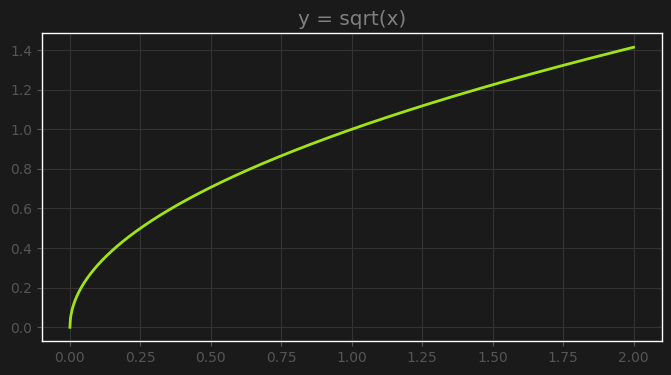
But looking closely we can see another characteristic of the square root curve that might not make it ideal for gradient descent. As the curve approaches zero, the gradient explodes to infinity. The derivative of $f(x)=\sqrt{x}$ is $f’(x)=\frac{1}{2\sqrt{x}}$, so we can see that at $x=0$ the gradient is infinite.
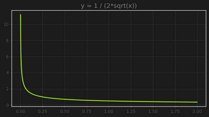
This indicates that as our loss approaches zero, the gradient will be so large that it will keep popping our weights away from their optimum values. To test this theory, we can try a toy example taking the root of mean absolute error, which is never done for reasons soon to become clear.
Let’s say we have a single model weight $m$, and a single observation $y=6$ associated with an input $x=3$. Clearly, the optimal solution is $m=2$, and any value above or below will scale the loss linearly with a constant slope of -3 or 3, as we can see here:
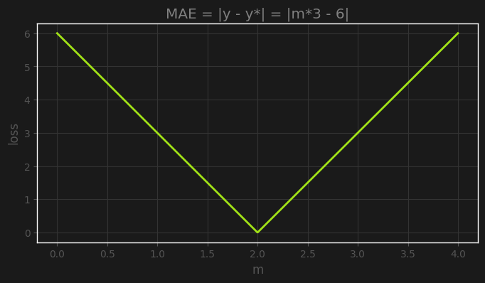
For our example, we’ll set a close initial estimate of $m=1.9$, a pretty small learning rate of 0.001 so that it is clear that what we observe is not being caused by choosing a large learning rate, and we’ll see what happens during 300 steps of gradient descent using MAE and RMAE as the training loss.
First, the gradient descent using MAE:
import matplotlib.pyplot as plt
import matplotlib.cm as cm

# Set variables
m = 1.9
x = 3
y = 6
lr = 0.001
n_iter = 300

# Set up plots
m_range = np.linspace(1.85, 2.15, 1000)
possible_losses = np.abs(m_range*3 - 6)
dot_colors = cm.gist_rainbow(np.linspace(0, 1, n_iter))
fig, axes = plt.subplots(3, figsize=(8,12), facecolor=(0.1, 0.1, 0.1))
_ = [(ax.set_facecolor((0.1, 0.1, 0.1)), ax.grid(color=(0.2, 0.2, 0.2))) for ax in axes]
axes[0].plot(m_range, possible_losses, linewidth=2, color="#a2e317")
for i, title in enumerate(["Loss curve", "current m", "absolute error"]):
    axes[i].set_title(title, color="gray")

# Gradient descent
for i in range(n_iter):
    derivative = m * (m*x - y) / np.abs(m*x - y)
    m -= lr * derivative
    pred = m * x
    loss = np.abs(pred - y)
    axes[0].scatter([m], [loss], color=dot_colors[i])
    axes[1].scatter([i], [m], color=dot_colors[i], s=1.5)
    axes[2].scatter([i], [loss], color=dot_colors[i], s=1.5)
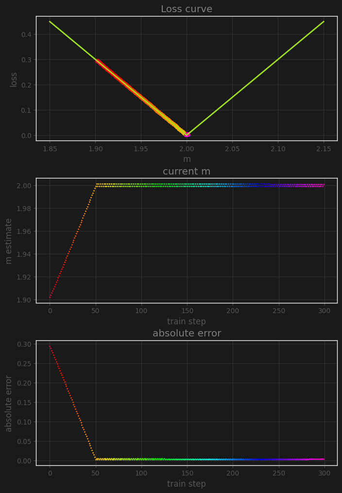
We can see in this example of the linear loss that the gradient descent process found the optimum, and stayed in that spot thanks to the small learning rate. Let’s see what happens if we repeat the same exact process, but use the root mean absolute error as training loss instead (keep in mind the plotted loss is still absolute error):
# Reset m value
m = 1.9

# Reset plots
fig, axes = plt.subplots(3, figsize=(8,12), facecolor=(0.1, 0.1, 0.1))
_ = [(ax.set_facecolor((0.1, 0.1, 0.1)), ax.grid(color=(0.2, 0.2, 0.2))) for ax in axes]
axes[0].plot(m_range, possible_losses, linewidth=2, color="#a2e317")
for i, title in enumerate(["Loss curve", "current m", "absolute error"]):
    axes[i].set_title(title, color="gray")

# Gradient descent
for i in range(n_iter):
    derivative = m * (m*x - y) / (2 * np.power(np.abs(m*x - y), 3/2))
    m -= lr * derivative
    pred = m * x
    loss = np.abs(pred - y)
    axes[0].scatter([m], [loss], color=dot_colors[i])
    axes[1].scatter([i], [m], color=dot_colors[i], s=2)
    axes[2].scatter([i], [loss], color=dot_colors[i], s=2)
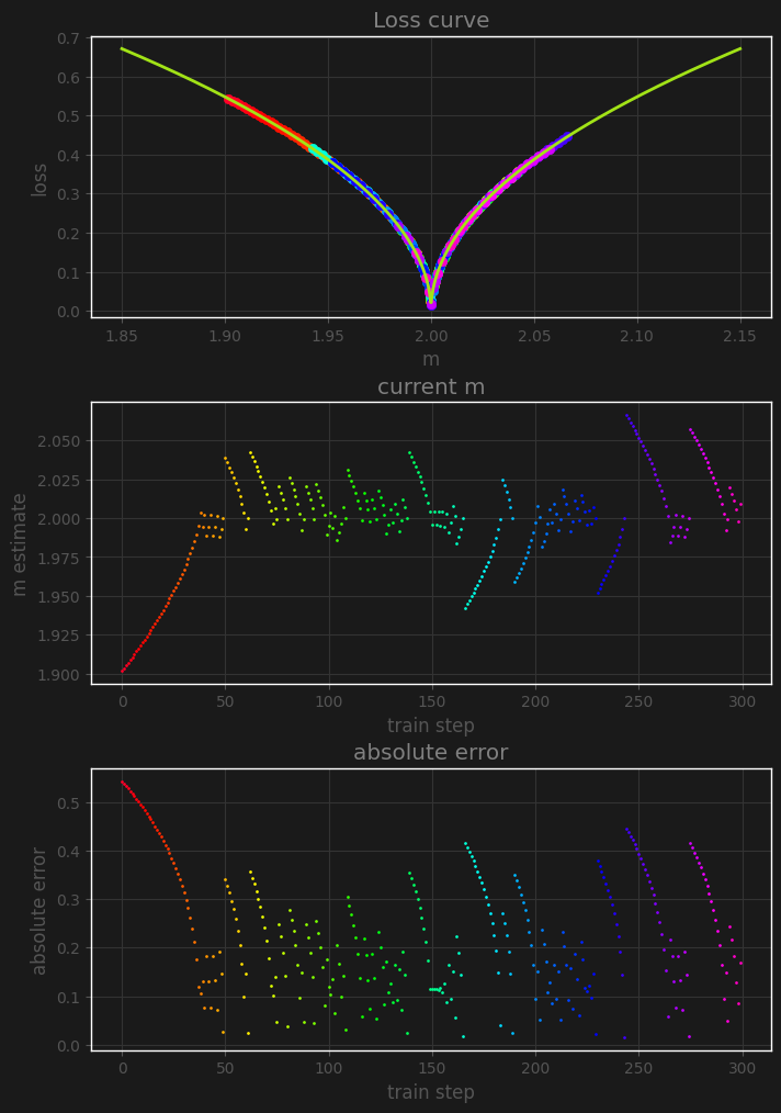
This time, we can see that every time the loss gets very close to zero, even our small learning rate can’t handle the massive gradients in that area, and the estimate gets popped far away from the optimum, even late in the training, leading to an unstable loss and parameter estimate.
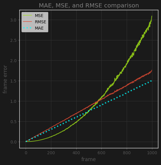
One might think: what about RMSE? It has a square root on top, does it have this problem? The answer is no, and it is easy to understand why. RMSE has a square root on top of already squared errors, which has taken the linear relationship of the depth difference and made it quadratic, so applying the square root on top actually cancels this out and takes it back to linear. The following example shows this:
gt = np.random.uniform(0, 5, 1000)
preds = np.array([gt + np.random.uniform(-i, i, 1000) for i in np.linspace(0, 3, 1000)])
errors = np.array(sorted(preds - gt, key=lambda x: np.abs(x).mean()))
mean_absolute_errors = np.abs(errors).mean(axis=1)
mean_squared_errors = np.power(errors, 2).mean(axis=1)
root_mean_squared_error = np.sqrt(mean_squared_errors)

fig, ax = plt.subplots(figsize=(6, 6), facecolor=(0.1, 0.1, 0.1))
ax.plot(mean_squared_errors, label="MSE", color="#a2e317", alpha=0.8)
ax.plot(root_mean_squared_error, label="RMSE", alpha=0.8)
ax.plot(mean_absolute_errors, color="cyan", linewidth=3, linestyle=":", label="MAE", alpha=0.8)
ax.set_title("MAE, MSE, and RMSE comparison", color="gray")
ax.set_facecolor((0.1, 0.1, 0.1))
ax.grid(color=(0.2, 0.2, 0.2))
ax.set_xlabel("frame")
ax.set_ylabel("frame error")
plt.legend();
Naturally, the follow-up question to this is: what does the distribution of SiLog error look like? Is it possible the square root is actually beneficial? We can’t answer this question without getting a look at what we’d be sending into the square root function, but luckily I have a recent Segformer for monocular depth training run where I was using SiLog loss without the square root on top, so we have a good sample of this distribution.
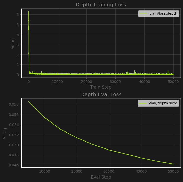
Above we can see the non-square root SiLog loss of the model over the first 50,000 training steps, using $\lambda=0.25$. Despite a low learning rate of 1e-5, the training loss converges very quickly thanks to pretrained weights to near zero, and from there the progress is mostly visible in the eval loss. We’ll focus on the train error after the curve dies down a bit to get a feel for what values would mostly be going through the square root function if we were using one:
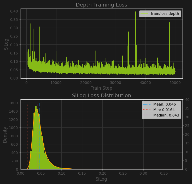
We can see that the majority of values are very close to zero, with a mean of 0.046, and a min value of 0.0164 in this sample. The gradient of a square root function is $f’(x)=\frac{1}{2\sqrt{x}}$, so for our minimum value of 0.0164, we would have a gradient of 3.904, which isn’t too scary, but maybe a bit higher than we would want for a near-zero loss, especially if we were multiplying it by $\alpha=10$ like in BTS.
While our loss value may not be getting close enough to zero to produce gradients near infinity, it does experience the highest gradients near the optimums, and I am skeptical that adding the square root on top of the SiLog loss function is a good idea. It isn’t going to be helping to reduce very large values given the nature of the inputs, and it has the potential to cause instability when losses approach zero.
That being said, it’s appropriate to run an experiment at this point to determine what the impact of the square root on the loss is on training, if there even is one. Below is a report on three training runs on the same training seed: one without square root, one with, and one without the square root, but higher learning rate. We see that despite the square root offering slightly better results due to generating higher gradients at near-zero loss, simply increasing the learning rate seems to be a better and more stable alternative. For this reason I conclude that for my own work, I won’t be using the square root of SiLog loss, but rather sticking to the equation offered in Eigen et al., 2014.